1 Joint Distribution

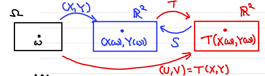
Now we want to explore multiple variables and their interaction. Here we focus on bivariate jointly continuous RVs.

A joint density function satisfies

• ${\displaystyle {\iint }_{{\mathbb{R}}^2}f(x,y)\mathrm{d}x\mathrm{d}y=1}$;
• ${\displaystyle f(x,y)\ge 0}$.

In the one dimensional case, for continuous RV, we have the approximation $$\mathbb{P}(X\in [x,x+\epsilon ))\approx f_X(x)\epsilon .$$
Similarly in two dimentional case, take a small neighborhood ${\displaystyle \mathrm{\Delta }}$ containing ${\displaystyle (x,y)}$, then we have $$\mathbb{P}((X,Y)\in \mathrm{\Delta })\approx f_{X,Y}\mathrm{Area}(\mathrm{\Delta }).$$

How to recover the marginal density ${\displaystyle f_X}$ or ${\displaystyle f_Y}$ given ${\displaystyle f_{X,Y}}$?

${\displaystyle X\stackrel{d}{=}W,Y\stackrel{d}{=}Z}$ will not lead to ${\displaystyle (X,Y)\stackrel{d}{=}(W,Z)}$: let ${\displaystyle X,W,V\stackrel{\mathrm{i}.\mathrm{i}.\mathrm{d}}{\sim }\mathrm{Exp}(1)}$, and ${\displaystyle Z\sim \mathrm{Gamma}(2,1)}$. Let ${\displaystyle Y=X+V}$. By this result we know ${\displaystyle Y\stackrel{\mathrm{d}}{\sim }\mathrm{Gamma}(2,1)}$. Then ${\displaystyle X\stackrel{\mathrm{d}}{=}W,Y\stackrel{\mathrm{d}}{=}Z}$. However, we always have ${\displaystyle X\le Y}$, and ${\displaystyle W>Z}$ has positive probability, so ${\displaystyle (X,Y)\stackrel{\mathrm{d}}{\ne }(W,Z)}$.

1.1 Independence

${\displaystyle X,Y}$ are independent if $$f_{X,Y}(x,y)=f_X(x)f_Y(y),\mathrm{\forall }(x,y)\in {\mathbb{R}}^2.$$
By independence, the value of ${\displaystyle X}$ will not give us anything about ${\displaystyle Y}$.

2 Bivariate Transformation

Transformation of random variables: ${\displaystyle T:{\mathbb{R}}^2\to {\mathbb{R}}^2,(X,Y)\mapsto (W,Z)}$.
Polar coordinates: ${\displaystyle (x,y)\mapsto (r,\theta ),x=r\cos \theta ,y=r\sin \theta }$.

Some properties:

• ${\displaystyle T}$ is invertible if and only if ${\displaystyle M_T}$ is invertible;
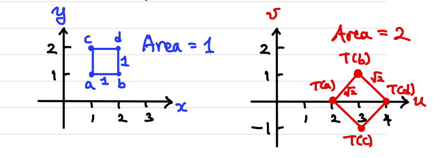
• ${\displaystyle P}$ is a parallelogram, then ${\displaystyle T(P)}$ is also one;
• ${\displaystyle \mathrm{Area}(T(P))=\mathrm{Area}(P)\cdot \det (M_T)}$.

Let ${\displaystyle T}$ be a linear transformation with inverse ${\displaystyle S}$. Given the joint p.d.f of ${\displaystyle (X,Y)}$, what's the joint p.d.f of ${\displaystyle (W,Z)=T(X,Y)}$?
On one hand, $$\mathbb{P}((W,Z)\in P)\approx f_{W,Z}(w,z)\mathrm{Area}(P).$$
Similarly $$\begin{array}{rl}\mathbb{P}((W,Z)\in P)& =\mathbb{P}(T(X,Y)\in P)=\mathbb{P}((X,Y)\in S(P))\\ & \approx f_{X,Y}(x,y)\mathrm{Area}(S(P))=f_{X,Y}(S(w,z))\mathrm{Area}(P)|det(M_S)|.\end{array}$$
We conclude that for invertible transformation ${\displaystyle T}$,

They preserve angles, lengths, Areas, ${\displaystyle \det (M_T)=\pm 1}$.

3 Invertible Affine Transformation

Suppose ${\displaystyle T:{\mathbb{R}}^2\to {\mathbb{R}}^2,T(X,Y)=(U,V)}$ has inverse ${\displaystyle S(U,V)=(X,Y)}$.

Define linear translation $$T(X,Y)=M_T\left[\begin{array}{c}X\\ Y\end{array}\right]+P_T=\left[\begin{array}{c}U\\ V\end{array}\right],$$ where ${\displaystyle M_T}$ is ${\displaystyle 2\times 2}$ invertible matrix, and ${\displaystyle P_T}$ is ${\displaystyle 2\times 1}$ vector.
Since ${\displaystyle ST(X,Y)=S(U,V)=(X,Y)}$, $$S(U,V)=M_T^{-1}\left[\begin{array}{c}U\\ V\end{array}\right]-M_T^{-1}{P}_T=M_S\left[\begin{array}{c}U\\ V\end{array}\right]+P_S.$$
Since $$\begin{array}{rl}\mathbb{P}((U,V)\in B)& =\mathbb{P}((X,Y)\in S(B))\\ \Rightarrow {\iint }_B{f}_{U,V}(u,v)\mathrm{d}u\mathrm{d}v& ={\iint }_{S(B)}{f}_{X,Y}(x,y)\mathrm{d}x\mathrm{d}y,\end{array}$$ we have $$\begin{array}{}\text{(3.1)}& f_{U,V}(u,v)=f_{X,Y}(S(u,v))|det{M}_S|.\end{array}$$

4 General Invertible Transformations

${\displaystyle T:{\mathbb{R}}^2\to {\mathbb{R}}^2}$. Assume differentiable, but not necessarily affine. Also assume ${\displaystyle T(X,Y)=(U,V)}$, ${\displaystyle S(U,V)=(X,Y)}$, ${\displaystyle ST(X,Y)=(X,Y)}$. So $$\begin{array}{rl}\mathbb{P}((U,V)\in \mathrm{\Delta })& =\mathbb{P}((X,Y)\in S(\mathrm{\Delta }))\\ \Rightarrow f_{U,V}(u,v)\mathrm{Area}(\mathrm{\Delta })& \approx f_{X,Y}(S(u,v))\mathrm{Area}(S(\mathrm{\Delta })).\end{array}$$
We want to know ${\displaystyle S(\mathrm{\Delta })}$.
If ${\displaystyle S}$ is affine, then ${\displaystyle S(\mathrm{\Delta })}$ is a parallelogram. For general ${\displaystyle S}$, if ${\displaystyle \delta ,\epsilon \ll 1}$, then ${\displaystyle S(\mathrm{\Delta })}$ can be approximated by a parallelogram, since ${\displaystyle S}$ can be approximated by an affine transformation on ${\displaystyle \mathrm{\Delta }}$.
Let $$S\left(\begin{array}{c}u\\ v\end{array}\right)=\left[\begin{array}{c}{S}_1(u,v)\\ S_2(u,v)\end{array}\right]\in {\mathbb{R}}^2,$$ where ${\displaystyle S_i:{\mathbb{R}}^2\to \mathbb{R},i=1,2}$ are differentiable functions. Then for any point ${\displaystyle (a,b)}$ near ${\displaystyle (u,v)}$, the Taylor expansion in second order gives $$S_i(a,b)\approx S_i(u,v)+(a-u)\frac{\partial S_i}{\partial u}(u,v)+(b-v)\frac{\partial S_i}{\partial v}(u,v).$$
In matrix notation, $$S\left[\begin{array}{c}a\\ b\end{array}\right]\approx \left[\begin{array}{c}{S}_1(u,v)\\ S_2(u,v)\end{array}\right]+\left[\begin{array}{cc}\frac{\partial S_1}{\partial u}(u,v)& \frac{\partial S_1}{\partial v}(u,v)\\ \frac{\partial S_2}{\partial u}(u,v)& \frac{\partial S_2}{\partial v}(u,v)\end{array}\right]\left[\begin{array}{c}a-u\\ b-v\end{array}\right].$$ This is an affine transformation. Denote the yellow matrix as ${\displaystyle J_S(u,v)}$, which is the Jacobian matrix of ${\displaystyle S}$ at ${\displaystyle (u,v)}$.

Hence, $$\mathbb{P}((X,Y)\in S(\mathrm{\Delta }))\approx f_{X,Y}(S(u,v))|det{J}_S(u,v)|\mathrm{Area}(\mathrm{\Delta }),$$ so $$\begin{array}{}\text{(4.1)}& f_{U,V}(u,v)=f_{X,Y}(S(u,v))|det{J}_S(u,v)|.\end{array}$$

In summary,

• ${\displaystyle X+Y\sim \mathrm{Gamma}({\alpha }_1+{\alpha }_2,\beta )}$,
• ${\displaystyle \frac{X}{X+Y}\sim \mathrm{Beta}({\alpha }_1,{\alpha }_2)}$,
• ${\displaystyle X+Y\perp \perp \frac{X}{X+Y}}$.